13.3. Properties of eigenfunctions

$\renewcommand{\Re}{\operatorname{Re}}$ $\renewcommand{\Im}{\operatorname{Im}}$ $\newcommand{\erf}{\operatorname{erf}}$ $\newcommand{\supp}{\operatorname{supp}}$ $\newcommand{\dag}{\dagger}$ $\newcommand{\const}{\mathrm{const}}$ $\newcommand{\mes}{\operatorname{mes}}$ ##[13.3. Properties of eigenfunctions](id:sect-13.3) ____________________________ > 1. [Base state](#sect-13.3.1) > 2. [Nodal sets](#sect-13.3.2) > 3. [Hearing the shape of the drum](#sect-13.3.3) ###[Base state](id:sect-13.3.1) We assume that $\Omega$ is connected domain. Consider the lowest eigenvalue $\lambda\_1$ and a corresponding eigenfunction $u\_1$. **[Theorem 1.](id:thm-13.3.1)** Let $\Omega $ be a connected domain. Then a. Eigenfunction $u\_1$ does not change its sign; b. $\lambda\_1$ is a simple eigenvalue. *Proof.* a. Let $v = |u\_1|$. Observe that $\\|v\\|=\\|u\_1\\|$ and $Q(v)=Q(u\_1)$. Then $|u\_1|=v$ is also an eigenfunction corresponding to eigenvalue $\lambda\_1$ and then $u\_{1,\pm}=\frac{1}{2}(|u\_1|\pm u\_1)=\max (\pm u\_1, 0)$ are also eigenfunctions corresponding to $\lambda_1$. At least one of these two eigenfunctions, say $u\_{1,+}$ is positive on some open set $\Omega'\subset \Omega$ and then $u\_{1,-}=0$ on $\Omega'$. However $(\Delta +\lambda\_1)u\_{1,-}=0$ and there are many different theorems implying that since $u\_{1,-}=0$ on $\Omega'$ it must be $0$ on $\Omega$. (For example: solutions of $(\Delta +\lambda\_1)v=0$ are analytic functions and there for analytic functions there is a unique continuation theorem.) Then $u\_1\ge 0$ in $\Omega$. b. If $u\_1$ and $v\_1$ are two linearly independent eigenfunctions corresponding to the same lowest eigenvalue $\lambda\_1$, then one can find $w\_1=u\_1+ \alpha u\_1$ which also is an eigenfunction and $(u\_1,w\_1)=0$ which is impossible since both of them have constant signs in $\Omega$ and therefore $u\_1w\_1$ has a constant sign in $\Omega$ and does not vanish identically in virtue of argument of (a). **[Remark 1.](id:remark-13.3.1)** a. Let $\lambda\_1\ge 0$. Assuming that $u\_1\ge 0$ we see that $u\_1$ is superharmonic function ($\Delta u\_1\le 0$) but such functions cannot reach minimum inside domain unless constant. So $u\_1>0$ in $\Omega$. b. Let $\lambda\_1<0$. Assuming that $u\_1\ge 0$ we see that $u\_1$ is subharmonic function ($\Delta u\_1\ge 0$) and such functions cannot reach maximum inside domain unless constant. c. While $\lambda\_1$ is always simple $\lambda\_n$ with $n\ge 2$ may be multiple. **[Corollary 1.](id:corollary-13.3.1)** $u\_n$ with $n\ge 2$ changes sign. Indeed, it is orthogonal to $u\_1$ which does not change a sign. ###[Nodal sets](id:sect-13.3.2) **[Definition 1.](id:definition-13.3.1)** Let $u\_n$ be an eigenfunction. Then $\\{x:\, u\_n(x)=0\\}$ is called a *nodal set* (*nodal line* as $d=2$) and connected components of $\\{x\in \Omega, u\_n(x)\ne 0\\}$ are called *nodal domains*. We know that for $n=1$ is just one nodal domain and for $n\ge 2$ there are at least 2 nodal domains. We need the following theorem from *Ordinary Differential Equations*: **[Theorem 2.](id:thm-13.3.2)** For $d=1$ there are exactly $n-1$ nodal points and $n$ nodal intervals for $u\_n$. **[Theorem 3.](id:thm-13.3.3)** For $d\ge 2$ if $u$ is an eigenfunction with an eigenvalue $\lambda\_n$ then $u\_n$ has no more than $n$ nodal domains. *Proof.* (i) Let $u$ have $m\ge n$ nodal domains. Consider $w\_k$ coinciding with $u$ in $k$-th nodal domain $\Omega\_k$ of $u$. Then $w\_1,\ldots, w\_m$ are linearly independent and \begin{gather\*} \\| c\_1w\_1+\ldots +c\_m w\_m\\|^2 = \sum\{1\le j\le m} c\_j^2 \\|w\_j\\|^2, \\\\ Q( c\_1w\_1+\ldots +c\_m w\_m) = \sum\{1\le j\le m} c\_j^2 Q(w\_j). \end{gather\*} Consider the space $L$ of linear combinations of $w\_1,\ldots, w\_m$ which are orthogonal to $u\_1,\ldots, u\_{n-1}$; then $L\ne \\{0\\}$. By definition $Q(v)\ge \lambda\_n \\|v\\|^2$ on $L$. Since $u\in L$ we conclude that $Q(u)\ge \lambda\_n \\|u\\|^2$; however $Q(u)=\lambda \\|u\\|^2$ and then $\lambda\ge \lambda\_n$. It proves theorem if $\lambda\_{n+1}>\lambda\_n$. Observe that since $(\Delta + \lambda\_n) w\_k=0$ in $\Omega\_k$ and $w\_k=0$ in $\Omega\setminus \Omega\_k$ we integrating by parts see that $Q(w\_k)=\lambda\_n\\|w\_k\\|^2$ for all $k$. Then $Q(v)=\lambda\_n\\|v\\|^2$ for all $v\in L$. Assume now that $m>n$. Then there exists $0\ne v\in L$ which is a linear combination of $w\_1,\ldots, w\_n$. Then $v$ is an eigenfunction but it is $0$ in $\Omega_{n+1}$ and therefore it must be $0$. Contradiction. Therefore if $\lambda\_{n-1}<\lambda\_n=\ldots =\lambda\_m$ then each eigenfunction corresponding to multiple eigenvalue $\lambda\_n$ has no more than $n$ nodal domains. Then we can use it in the case when variables are separated (we consider only $d=2$ and only Dirichlet boundary condition: **[Example 1.](id:example-13.3.1)** Let $\Omega=\\{0< x< a, 0 < y < b\\}$ be a rectangular box. Let us separate variables; then \begin{equation} u\_{pq}=\sin \Bigl(\frac{p\pi x}{a}\Bigr) \sin \Bigl(\frac{q\pi y}{b}\Bigr),\qquad \mu\_{pq}= \pi^2 \Bigl(\frac{p^2}{a^2}+\frac{q^2}{b^2}\Bigr). 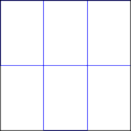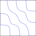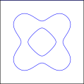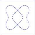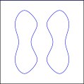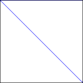\label{eq-13.3.1} \end{equation} Then nodal lines form a rectangular grid (see below). Let $a=b=\pi$. 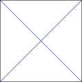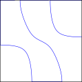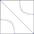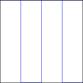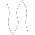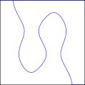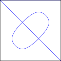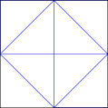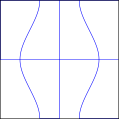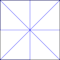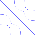a. Then $\lambda\_1=2$ and $\lambda\_2=\lambda\_3=10$ (where $\lambda\_n$ are $\mu\_{pq}$ ordered). First figure shows nodal lines for $u\_{21}$ (and nodal lines for $u\_{12}$ are exactly like this but flipped over $x=y$). Consider now linear combinations of $u\_{21}$ and $u\_{12}$:


$u_{21}$	$u_{21}+\frac{1}{2} u_{12}$	$u_{21}+u_{12}$

b. Next $\lambda\_4=8$:

$u_{22}$

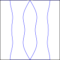
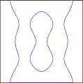
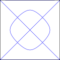
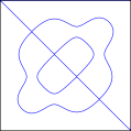
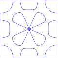
c. Further $\lambda\_5=\lambda\_6=10$. First figure shows nodal lines for $u\_{31}$ (and nodal lines for $u\_{13}$ are exactly like this but flipped over $x=y$). Consider now linear combinations of $u\_{31}$ and $u\_{13}$:


$u_{31}$	$u_{31}+u_{13}$	$u_{31}+\frac{1}{3}u_{13}$	$u_{31}-\frac{1}{3}u_{13}$	$u_{31}-u_{13}$

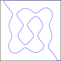
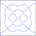
Comparing two last pictures we see that crossing open under small perturbations. d. Further $\lambda\_7=\lambda\_8=13$, First figure shows nodal lines for $u\_{32}$ (and nodal lines for $u\_{23}$ are exactly like this but flipped over $x=y$). Consider now linear combinations of $u\_{32}$ and $u\_{23}$:


$u_{32}$	$u_{32}+\frac{1}{2}u_{23}$	$u_{32}+u_{23}$

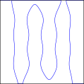
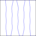
e. Further $\lambda\_9=\lambda\_{10}=17$, First figure shows nodal lines for $u\_{41}$ (and nodal lines for $u\_{14}$ are exactly like this but flipped over $x=y$). Consider now linear combinations of $u\_{412}$ and $u\_{14}$:


$u_{41}$	$u_{41}+\sqrt{\frac{2}{27}}u_{14}$	$u_{41}+{\frac{1}{2}}u_{14}$	$u_{41}+u_{14}$

f. Further $\lambda\_{11}=18$ is simple $p=q=3$ and thus trivial; furthermore $\lambda\_{12}=\lambda\_{13}=20$ with $p=4, q=2$ is also trivial: we need just to take any picture for $p=2,q=1$ and make its double mirror reflection arriving to


$u_{42}+u_{24}$	$u_{42}+\frac{1}{2}u_{24}$	$u_{42}-u_{24}$

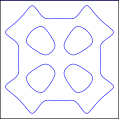
and similar pictures (we do not draw $u\_{pq}$ anymore). f. Further $\lambda\_{14}=\lambda\_{15}=25$ does not produce anything much different from (d) but simply more nodal domains:


$u_{43}+u_{34}$	$u_{43}+\frac{1}{2}u_{34}$

g. Further $\lambda\_{16}=\lambda\_{17}=26$:


$u_{51}+u_{15}$	$u_{51}+\frac{4}{5}u_{15}$	$u_{51}+\frac{1}{2}u_{15}$	$u_{51}+\frac{1}{4}u_{15}$

$u_{51}-\frac{1}{5}u_{15}$	$u_{51}-\frac{1}{2}u_{15}$	$u_{51}-u_{15}$

h. Skipping $\lambda\_{18}=\lambda\_{19}=29$, $\lambda\_{20}=32$, $\lambda\_{21}=\lambda\_{22}=34$, consider $\lambda\_{23}=\lambda\_{24}=37$


$u_{61}+u_{16}$	$u_{61}+\frac{4}{5}u_{16}$	$u_{61}+\frac{1}{5}u_{16}$	$u_{61}+\frac{1}{10}u_{16}$

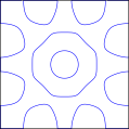
i. Starting from $\lambda=50=7^2+1^2=5^2+5^2$ multiplicities could be larger than $2$ and the following gallery is just a tiny sample

**[Example 2.](id:example-13.3.2)** Consider $\Omega=\\{ 0< y < x <\pi\\}$ which is a triangle. a. If on the diagonal $x=y$ a Dirichlet condition is required, then eigenfunctions are $u\_{pq}(x,y)-u\_{pq}(y,x)$ with $p\ne q$ (or their linear combination like $u\_{83}(x,y)-u\_{83}(y,x)$ and $u\_{74}(x,y)-u\_{74}(y,x)$). b. If on the diagonal $x=y$ a Neumann condition is required, then eigenfunctions are $u\_{pq}(x,y)+u\_{pq}(y,x)$ (or their linear combination like $u\_{71}(x,y)+u\_{71}(y,x)$ and $u\_{55}(x,y)$). 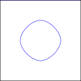**[Example 3.](id:example-13.3.3)** a. Let $\Omega=\\{r\le b \\}$ be a disk. Then nodal lines form a circular grid: $u\_{pq}(r,\theta)= \cos (p\theta) J\_{p}(k\_{pq}r)$ where $J\_p(z)$ are Bessel functions and $k\_{pq} b$ is $q$-th root of $J\_p(z)$. The similar statement is true for circular sectors, rings etc. 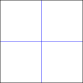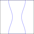b. Let $\Omega$ be an ellipse. Then (see [Subsection 6.3.3](../S6.3.html#sect-6.3.3)) in the elliptical coordinates Laplacian is \begin{equation} \Delta = \frac{1}{c^2\bigl(\sinh^2(\sigma)+\sin^2(\tau) \bigr)} (\partial\_\sigma^2 +\partial\_\tau^2 ) \label{eq-13.3.2} \end{equation} and separating variables $u= S(\sigma)T(\tau)$ we get \begin{align} & S'' +\bigl( \lambda c^2 \sinh^2(\sigma) -k\bigr)S=0,\label{eq-13.3.3}\\\\ & T'' + \bigl( \lambda c^2 \sin^2(\tau) + k\bigr)T=0.\label{eq-13.3.4} \end{align} For $T$ we have either $\pi$-periodic or $\pi$-antiperiodic boundary condition: $T(\tau +\pi)=\pm T(\tau)$ and for $S$ we have Dirichlet boundary condition as $\cosh (\sigma)= a/c$ and respectively Neumann and Dirichlet boundary condition as $\sigma=0$ arising from $S(\pm \sigma)= \pm S(\sigma)$. So we have a grid consisting from confocal ellipses and hyperbolas. The similar statement is true for elliptical "sectors", rings etc. 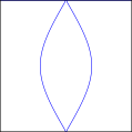c. Let $\Omega$ be an parabolic lense. Then (see [Subsection 6.3.3](../S6.3.html#sect-6.3.3)) in the parabolic coordinates \begin{equation} \Delta = \frac{1}{\sigma^2+\tau^2} (\partial\_\sigma^2 +\partial\_\tau^2 ) \label{eq-13.3.5} \end{equation} and separating variables $u= S(\sigma)T(\tau)$ we get \begin{align} & S'' +\bigl( \lambda \sigma^2 -k\bigr)S=0,\label{eq-13.3.6}\\\\ & T'' + \bigl( \lambda c^2 \tau^2 + k\bigr)T=0.\label{eq-13.3.7} \end{align} So we have a grid consisting from confocal parabolas. **[Remark 2.](id:remark-13.3.2)** For generic domais (any sufficiently small perturbation of generic domain is a generic domain again but an arbitrarily small perturbation of non-generic domain may result in generic domain) a. All eigenvalues are simple; b. Nodal lines do not have self-intersections. **[Remark 3.](id:remark-13.3.3)** Historically interest to nodal lines appeared from [Chladni plates](http://en.wikipedia.org/wiki/Ernst_Chladni) but those are nodal lines for biharmonic operator \begin{equation} (\Delta ^2-\lambda )u=0 \label{eq-13.3.8} \end{equation} with free boundary conditions (appearing from variational problem \begin{equation} \delta \Bigl (\iint \bigl(u\_{xx}^2+ 2u\_{xy}^2 + u\_{yy}^2 -\lambda u^2\bigr)\,dxdy\Bigr)=0 \label{eq-13.3.9} \end{equation} (without boundary conditions). This is much more complicated question which was (partially) solved by [Marie-Sophie Germain](http://en.wikipedia.org/wiki/Sophie_Germain). ###[Hearing the shape of the drum](id:sect-13.3.3) In 1965(?) Marc Kac asked the question"Can one hear the shape of the drum" which meant: if we know all the eigenvalues of the Dirichlet Laplacian $\Delta$: $0<\lambda\_1 <\lambda\_2 \le \lambda\_3\le \ldots $ in the connected domain $\Omega$, can we restore $\Omega$ (up to isometric movements—shift and rotations). The extensive study was using the method of *spectral invariants*, which are numbers which have some geometric meaning and which can be calculated from $0<\lambda\_1 <\lambda\_2 \le \lambda\_3\le \ldots $. The main source of such invariants was the *method of heat equation*: Namely let $G(x,y,t)$ with $x,y\in \Omega$ and $t>0$ be a Green function: \begin{align} &G\_t -\Delta\_x G=0,\label{eq-13.3.10}\\\\ &G|_{t=0}=\delta (x-y),\label{eq-13.3.11}\\\\ &G|\_{x\in \partial \Omega}=0\label{eq-13.3.12} \end{align} and let \begin{equation} \sigma(t)= \iint u(x,x,t)\, dx= \sum\_{n\ge 1} e^{-\lambda\_n t} \label{eq-13.3.13} \end{equation} be a *heat trace*; then \begin{equation} \sigma(t)\sim \sum \_{k\ge -d} c\_k t^{k}\qquad \text{as }\ t\to +0 \label{eq-13.3.14} \end{equation} **Check!** where $c\_k$ are heat invariants. It was proven that (as $d=2$, for $d\ge 3$ similarly) area, perimeter, number of holes and many other geometric characteristic are spectral invariants but the final answer was negative: there are *isospectral* domains $\Omega$ and $\Omega'$ (so that eigenvalues of Laplacians in those are equal) which are not *isometric* (have different shapes). --------------- [$\Leftarrow$](./S13.2.html) [$\Uparrow$](../contents.html) [$\Rightarrow$](./S13.4.html)