$\renewcommand{\Re}{\operatorname{Re}}$
$\renewcommand{\Im}{\operatorname{Im}}$
$\newcommand{\erf}{\operatorname{erf}}$
$\newcommand{\dag}{\dagger}$
$\newcommand{\const}{\mathrm{const}}$
$\newcommand{\arcsinh}{\operatorname{arcsinh}}$
##[3.2. Heat equation (Miscellaneous)](id:sect-3.2)
----------------
> 1. [1D Heat equation on half-line](#sect-3.2.1)
> 2. [Inhomogeneous boundary conditions](#sect-3.2.2)
> 3. [Inhomogeneous right-hand expression](#sect-3.2.3)
> 4. [Multidimensional heat equation](#sect-3.2.4)
> 5. [Maximum principle](#sect-3.2.5)
> 6. [References](#sect-3.2.6)
###[1D Heat equation on half-line](id:sect-3.2.1)
In the previous section we considered heat equation
\begin{equation}
u\_t=ku\_{xx}
\label{eq-3.2.1}
\end{equation}
with $x\in \mathbb{R}$ and $t\>0$ and derived formula
\begin{equation}
u(x,t)=\int
\_{-\infty}^\infty G(x,y,t) g(y)\,dy.
\label{eq-3.2.2}
\end{equation}
with
\begin{equation}
G(x,y,t)=G\_0(x-y,t):=
\frac{1}{2\sqrt{k\pi t}}e^{-\frac{(x-y)^2}{4kt}}
\label{eq-3.2.3} \end{equation} for solution of IVP $u|\_{t=0}=g(x)$.
Recall that $G(x,y,t)$ quickly decays as $|x-y|\to \infty$ and it
tends to $0$ as $t\to +0$ for $x\ne y$, but $\int G(x,y,t)\,dy=1$.
Consider the same equation (\ref{eq-3.2.1}) on half-line with the homogeneous Dirichlet or Neumann boundary condition at $x=0$:
the method of continuation
\begin{align}
&u\_D|\_{x=0}=0,\tag{D}\label{eq-3.2.D}\\\\[3pt]
&u\_{N\,x}|\_{x=0}=0\tag{N}.\label{eq-3.2.N}
\end{align}
This solution also has a form (\ref{eq-3.2.2}) but with different function $G(x,y)$ (and obviously with the different domain of integration $[0,\infty)$):
\begin{align}
&G=G\_D(x,y,t)=G\_0(x-y,t)-G\_0(x+y,t),\label{eq-3.2.4}\\\\[3pt]
&G=G\_Nx,y,t)|=G\_0(x-y,t)+G\_0(x+y,t)\label{eq-3.2.5}
\end{align}
for (\ref{eq-3.2.D}) and (\ref{eq-3.2.N}) respectively.
Both these functions satisfy equation (\ref{eq-3.2.1}) with respect to $(x,t)$,
\begin{align}
&G\_D|\_{x=0}=0,\label{eq-3.2.6}\\\\[3pt]
&G\_{N\,x}|\_{x=0}=0.\label{eq-3.2.7}
\end{align}
tend to $0$ as $t\to +0$, $x\ne y$
\begin{align}
&\int\_0^\infty G\_D(x,y,t)\,dy\to 1
\qquad \text{as }t\to+0,\label{eq-3.2.8}\\\\[3pt]
&\int\_0^\infty G\_D(x,y,t)\,dx= 1.\label{eq-3.2.9}
\end{align}
Further,
\begin{equation}
G(x,y,t)=G(y,x,t)
\label{eq-3.2.10}
\end{equation}
One can prove it by the method of continuation. Indeed, coefficients do not depend on $x$ and equation contains only even order derivatives with respect to $x$. Recall from [Subsection 2.6.3](../Chapter2/S2.6.html#sect-2.6.3) that continuation is even under Neumann condition and odd under Dirichled condition.
###[Inhomogeneous boundary conditions](id:sect-3.2.2)
Consider now inhomogeneous boundary conditions
\begin{align}
&u\_D|\_{x=0}=p(t),\label{eq-3.2.11}\\\\[3pt]
&u\_{N\,x}|\_{x=0}=q(t).\label{eq-3.2.12}
\end{align}
Consider
\begin{equation\*}
0=\int\_\Pi G(x,y,t-\tau)
\bigl(-u\_{\tau}(y,\tau)+ku\_{yy}(y,\tau)\bigr)\,d\tau'dy
\end{equation\*}
with $\Pi=\\{x\>0, 0\< \tau \< t-\epsilon \\}$.
Integrating by parts with respect to $\tau$ in the first term and twice with respect to $y$ in the second one we get
\begin{align\*}
0=&\int\_\Pi \bigl( -G\_t (x,y,t-\tau) + k
G\_{yy}(x,y,t-\tau)\bigr)u(y,\tau)\,d\tau'dy\\\\
-& \int\_0^\infty
G (x,y,\epsilon) u(y,t-\epsilon)\, dy +
\int \_0^\infty G (x,y,t) u(y,0)\, dy+ \\\\
& k \int\_0^{t-\epsilon} \bigl( -G(x,y,t-\tau)u\_y(y,\tau) +
G\_y(x,y,t-\tau)u(y,\tau)\bigr)\_{y=0}\,d\tau.
\end{align\*}
Note that, since $G$ satisfies (\ref{eq-3.2.1}) with respect to $(y,t)$ as
well due to symmetry, the first line is $0$.
In the second line the first term tends to $-u(x,t)$ because of properties of $G(x,y,t)$ (really, tends everywhere but for $x=y$ to $0$ and its integral from $0$ to $\infty$ tends to $1$).
So we get
\begin{multline}
u(x,t)=\int\_0^\infty G(x,y,t)\underbrace{u(y,0)}\_{=g(y)}\,dy+\\\\
\int\_0^{t} \bigl( -G(x,y,t-\tau)u\_y(y,\tau) +
G\_y(x,y,t-\tau)u(y,\tau)\bigr)\_{y=0}\,d\tau.
\qquad
\label{eq-3.2.13}
\end{multline}
The first line gives in the r.h.e. us solution of the IBVP with $0$ boundary condition. Let us consider the second line.
In the case of Dirichlet boundary condition $G(x,y,t)=0$ as $y=0$
and therefore we get here
\begin{equation\*}
k \int\_0^{t} G\_y(x,y,t-\tau)\underbrace{u(0,\tau)}\_{=p(\tau)}\,d\tau;
\end{equation\*} In the case of Neumann boundary condition
$G\_y(x,y,t)=0$ as $y=0$ and therefore we get here
\begin{equation\*}
-k \int\_0^{t} G(x,y,t-\tau)\underbrace{u(0,\tau)}\_{=q(\tau)}\,d\tau.
\end{equation\*}
So, (\ref{eq-3.2.13}) becomes
\begin{equation}
u\_D(x,t)=\int\_0^\infty G\_D(x,y,t)g(y)\,dy+k
\int\_0^{t} G\_{D\,y}(x,0,t-\tau)p(\tau) \,d\tau; \qquad \label{eq-3.2.14}
\end{equation}
and
\begin{equation}
u\_N(x,t)=\int\_0^\infty G\_N(x,y,t)g(y)\,dy-
k \int\_0^{t} G\_{N\,y}(x,0,t-\tau)q(\tau) \,d\tau.\qquad
\label{eq-3.2.15} \end{equation}
->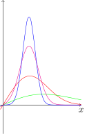 <-
Plots of $G\_{D}(x,y,t)$ and $G\_{N}(x,y,t)$ as $y=0$ (for some values of $t$)
**[Remark 1.](id:remark-3.2.1)**
a. If we consider a half-line $(-\infty,0)$ rather than
$(0,\infty)$ then the same terms appear on the right end
($x=0$) albeit with the opposite sign;
b. If we consider a finite interval $(a,b)$ then there will be
contributions from both ends;
c. If we consider Robin boundary condition $(u\_x-\alpha
u)|\_{x=0}=q(t)$ then formula (\ref{eq-3.2.15}) would work but $G$
should satisfy the same Robin condition and we cannot consruct $G$
by a method of continuation.
###[Inhomogeneous right-hand expression](id:sect-3.2.3)
Consider equation
\begin{equation}
u\_t-ku\_{xx}=f(x,t).
\label{eq-3.2.16}
\end{equation}
Either by Duhamel principle or just using the same calculations as above one can prove that its contribution would be
\begin{equation}
\int\_0^t \int G(x,y,t-\tau) f(y,\tau)\,dyd\tau
\label{eq-3.2.17}
\end{equation}
with the same $G$ as was used for equation (\ref{eq-3.2.1}).
###[Multidimensional heat equation](id:sect-3.2.4)
Now we claim that for 2D and 3D heat equations
\begin{align}
&u\_t=k\bigl(u\_{xx}+u\_{yy}\bigr), \label{eq-3.2.18}\\\\
&u\_t=k\bigl(u\_{xx}+u\_{yy}+u\_{zz}\bigr), \label{eq-3.2.19}
\end{align}
similar formulae hold:
\begin{align}
&u=\iint G\_2 (x,y;x',y';t) g(x',y')\,dx'dy', \label{eq-3.2.20}\\\\
&u=\iiint G\_3 (x,y,z;x',y',z';t) g(x',y',z')\,dx'dy'dz' \label{eq-3.2.21} \end{align}
with
\begin{align}
&G\_2 (x,y;x',y';t) =&& G\_1(x,x',t)G\_1(y,y',t), \label{eq-3.2.22}\\\\
&G\_3 (x,y,z;x',y',z';t) =&& G\_1(x,x',t)G\_1(y,y',t)G\_1(z,z',t);
\label{eq-3.2.23}
\end{align}
in particular for the whole $\mathbb{R}^n$
\begin{align} &G\_n (\mathbf{x},\mathbf{x}';t) =&&
(2\sqrt{\pi k t})^{-n/2}e^{-\frac{|\mathbf{x}-\mathbf{x}'|}{4kt}}. \label{eq-3.2.24}
\end{align}
To justify our claim we note that
a. $G\_n$ satisfies $n$-dimensional heat equation. Really, consider
f.e. $G\_2$: \begin{align\*} G\_{2\,t} (x,y;x',y';t) =&
G\_{1\,t}(x,x',t)G\_1(y,y',t)+G\_1(x,x',t)G\_{1.t}(y,y',t)=\\\\ &
kG\_{1\,xx}(x,x',t)G\_1(y,y',t)+kG\_1(x,x',t)G\_{1\,yy}(y,y',t)=\\\\
&k \Delta \bigl( G\_{1\,t}(x,x',t)G\_1(y,y',t) \bigr)= k\Delta
G\_2(x,y;x',y';t) \end{align\*}
b. $G\_n (\mathbf{x},\mathbf{x}';t)$ quickly decays as
$|\mathbf{x}-\mathbf{x}'|\to \infty$ and it tends to $0$ as
$t\to +0$ for $\mathbf{x}\ne \mathbf{x}'$, but
c. $\int G(\mathbf{x},\mathbf{x}',t)\,dy\to 1$ as $t\to +0$;
d. $G(\mathbf{x},\mathbf{x}',t)=G(\mathbf{x}',\mathbf{x},t)$.
The last three properties are due to the similar properties of $G\_1$.
Properties (a)-(d) imply integral representation (\ref{eq-3.2.20}) (or its
$n$-dimensional variant).
###[Maximum principle](id:sect-3.2.5)
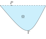
Consider heat eqution in the domain $\Omega$ like below
-><-
We claim that
**[Proposition 1.](id:prop-3.2.1)(maximum principle).**
Let $u$ satisfy heat equation in $\Omega$. Then
\begin{equation} \max \_\Omega u = \max \_\Gamma u.
\label{eq-3.2.25}
\end{equation}
*Almost correct proof.* Let (\ref{eq-3.2.25}) be wrong. Then there exist point $P=(\bar{x},\bar{t})\in \Omega\setminus \Gamma$ s.t. $u$ reaches its maximum at $P$. Without any loss of the generality we can assume that $P$ belongs to an upper lid of $\Omega$. Then
\begin{equation}
u\_t(P )\ge 0 \label{eq-3.2.26}
\end{equation}
(really
$u(\bar{x},\bar{t})\ge u(\bar{x},t)$ for all $t: \bar{t}\>t\>\bar{t}-\epsilon$ and then $\bigl( u(\bar{x},\bar{t})-u(\bar{x},t)\bigr)/(\bar{t}-t)\ge 0$ and as
$t\nearrow \bar{t}$) we get (\ref{eq-3.2.26}).
Also $u\_{xx}( P)\le 0$ (really $u(x,\bar{t})$ reaches maximum as $x=\bar{x}$). This inequality combined with (\ref{eq-3.2.26}) almost contradict to heat equation (*almost* because there could be equalities).
*Correct proof.* Note first that the above arguments prove (\ref{eq-3.2.25}) if $u$ satisfies inequality $u\_t-ku\_{xx}\<0$ because then there will be contradiction.
Note that $v= u-\varepsilon t$ satisfies $v\_t-kv\_{xx}\<0$ for any
$\varepsilon \>0$ and therefore
\begin{equation\*}
\max \_\Omega (u-\varepsilon t) = \max \_\Gamma (u-\varepsilon t).
\end{equation\*}
Taking limit as $\varepsilon \to +0$ we get (\ref{eq-3.2.25}).
**[Remark 2.](id:remark-3.2.2)**
a. Sure, the same proof works for multidimensional heat equation.
b. In fact, *either* in $\Omega \setminus \Gamma$ $u$ is strictly less than
$\max \_\Gamma u$ *or* $u=\const$. The proof is a bit more sophisticated.
**[Corollary 1.](id:corollary-3.2.1) (minimum principle)**
\begin{equation}
\min \_\Omega u = \min \_\Gamma u. \label{eq-3.2.30}
\end{equation}
Really, $-u$ also satisfies heat equation.
**[Corollary 2.](id:corollary-3.2.2)**
$u=0$ everywhere on $\Gamma$ $\implies u=0$ everywhere on $\Omega$.
Really, then $\max \_\Omega u=\min\_\Omega u=0$.
**[Corollary 3.](id:corollary-3.2.3)**
Let $u,v$ both satisfy heat equation. Then $u=v$ everywhere on $\Gamma$ $\implies u=v$ everywhere on $\Omega$.
*Proof.*
Really, then $(u-v)$ satisfies heat equation.
###[References](id:sect-3.2.6)
1. [erf
function](http://www.wolframalpha.com/input/?i=erf%28x%29&lk=4#=1)
2. [erf
derivative](http://www.wolframalpha.com/input/?i=%28erf%28x%29%29%27)
---------------
[$\Leftarrow$](S3.1.html) [$\Uparrow$](../contents.html) [$\downarrow$](./S3.2.P.html) [$\Rightarrow$](./S3.A.html)