< $\renewcommand{\Re}{\operatorname{Re}}$ $\renewcommand{\Im}{\operatorname{Im}}$ $\newcommand{\erf}{\operatorname{erf}}$ $\newcommand{\dag}{\dagger}$ $\newcommand{\const}{\mathrm{const}}$ $\newcommand{\arcsinh}{\operatorname{arcsinh}}$ ##[9.2. Wave equation: energy method](id:sect-9.2) ------------- > 1. [Energy method: local for](#sect-9.2.1) > 2. [Classification of hypersurfaces](#sect-9.2.2) > 3. [Application to Cauchy problem](#sect-9.2.3) > 4. [Application to IBVP](#sect-9.2.4) > 5. [Remarks](#sect-9.2.5) ###[Energy method: local form](id:sect-9.2.1) Consider wave equation \begin{equation} u\_{tt}-c^2\Delta u=0. \label{eq-9.2.1} \end{equation} Multiplying by $u\_t$ we arrive to \begin{multline\*} 0=u\_t u\_{tt}-c^2 u\_t\Delta u= \frac{1}{2}\partial\_t (u\_{t}^2)-c^2\nabla \cdot (u\_t\nabla u) + c^2\nabla u\_t \cdot \nabla u =\\\\ \frac{1}{2}\partial\_t \bigl(u\_{t}^2+c^2|\nabla u|^2\bigr)- c^2\nabla \cdot (u\_t\nabla u) \end{multline\*} that is \begin{equation} \frac{1}{2}\partial\_t \bigl(u\_{t}^2+c^2|\nabla u|^2\bigr)- c^2\nabla \cdot (u\_t\nabla u)=0. \label{eq-9.2.2} \end{equation} This is an *energy conservation law in the local form*. If we integrate over domain $\Omega\subset \mathbb{R}\_t\times \mathbb{R}\_x^n$ we arrive to \begin{equation} \iint\_{\Sigma} \Bigl( \bigl(u\_{t}^2+|\nabla u|^2\bigr)\nu\_t -c^2 u\_t \nabla u \cdot \nu\_x\Bigr) \,d\sigma=0 \label{eq-9.2.3} \end{equation} where $\Sigma$ is a boundary of $\Omega$, $\nu$ is an external normal and $d\sigma$ is an alement of "area"; $\nu\_t$ and $\nu\_x$ are its $t$ and $x$ components. ###[Classification of hypersurfaces](id:sect-9.2.2) Consider a quadratic form \begin{equation} Q(U\_0,\mathbf{U})=U\_0^2 +|\mathbf{U}|^2 - 2U\_0 c\nu\_t^{-1}\nu\_x\cdot \mathbf{U}. \label{eq-9.2.4} \end{equation} **[Proposition 1.](id:prop-9.2.1)** a. If $c|\nu\_x|\<|\nu\_t|$ then $Q$ is positive definite (i.e. $Q(U\_0,\mathbf{U})\ge 0$ and $Q(U\_0,\mathbf{U})=0$ iff $U\_0=\mathbf{U}=0$); b. If $c|\nu\_x|=|\nu\_t|$ then $Q$ is non-negative definite (i.e. $Q(U\_0,\mathbf{U})\ge 0$); c. If $c|\nu\_x|\>|\nu\_t|$ then $Q$ is not non-negative definite. *Proof* is obvious. **[Definition 1.](id:definition-9.2.1)** a. If $c|\nu\_x|\<|\nu\_t|$ then $\Sigma$ is a *space-like surface* (in the given point). b. If $c|\nu\_x|=|\nu\_t|$ then $\Sigma$ is a *characteristic* (in the given point). c. If $c|\nu\_x|\>|\nu\_t|$ then $\Sigma$ is a *time-like surface* (in the given point). **[Remark 1.](id:remark-9.2.1)** Those who studied special relativity can explain (a), (c). 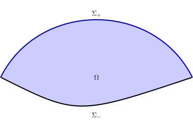###[Application to Cauchy problem](id:sect-9.2.3) Consider now bounded domain $\Omega$ bounded by $\Sigma=\Sigma\_+\cup\Sigma\_-$ where $c|\nu\_x|\le -\nu\_t$ at each point of $\Sigma\_-$ and $c|\nu\_x|\le \nu\_t$ at each point of $\Sigma\_+$. Assume that $u$ satisfies (\ref{eq-9.2.1}) \begin{equation} u=u\_t=0 \qquad \text{on }\ \Sigma\_-. \label{eq-9.2.5} \end{equation} Then (\ref{eq-9.2.3}) implies that \begin{equation\*} \iint\_{\Sigma\_+} \Bigl(\bigl(u\_{t}^2+|\nabla u|^2\bigr)\nu\_t - c^2 u\_t \nabla u \cdot \nu\_x\Bigr)\,d\sigma=0 \end{equation\*} which due to assumption about $\Sigma\_+$ implies that integrand is $0$ and therefore $u\_t=\nabla u=0$ in each point where $c|\nu\_x|\<\nu\_t$. -><- We can apply the same arguments to $\Omega\_T:=\Omega \cap \\{t\< T\\}$ with the boundary $\Sigma\_T= \Sigma \cap \\{t\< T\\}\cup S\_T$, $S\_T:=\Omega\cap\\{t=T\\}$; note that on $S\_T$ $\nu\_t=1$, $\nu\_x=0$. 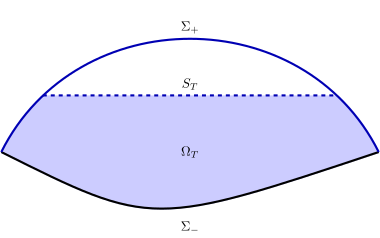-><- Therefore $u\_t=\nabla u=0$ on $S\_T$ and since we can select $T$ arbitrarily we conclude that this is true everywhere in $\Omega$. Since $u=0$ on $\Sigma\_-$ we conclude that $u=0$ in $\Omega$. So we proved: **[Theorem 1.](id:thm-9.2.1)** Consider a bounded domain $\Omega$ bounded by $\Sigma=\Sigma\_+\cup\Sigma\_-$ where $c|\nu\_x|\le -\nu\_t$ at each point of $\Sigma\_-$ and $c|\nu\_x|\le \nu\_t$ at each point of $\Sigma\_+$. Assume that $u$ satisfies (\ref{eq-9.2.1}), (\ref{eq-9.2.5}). Then $u=0$ in $\Omega$. It allows us to prove **[Theorem 2.](id:thm-9.2.2)** Consider $(y,\tau)$ with $\tau\>0$ and let $K^-(y,\tau)= \\{(x,t): t\le \tau, |y-x|\< c(\tau-t)\\}$ be a *backward light cone* issued from $(y,\tau)$. Let a. $u$ satisfy (\ref{eq-9.2.1}) in $K^-(y,\tau)\cap \\{t\>0\\}$, b. $u=u\_t=0$ at $K^-(y,\tau)\cap \\{t=0\\}$. Then $u=0$ in $K^-(x,t)\cap \\{t\>0\\}$. *Proof* is obvious: we can use $\Omega=K^-(x,t)\cap \\{t\>0\\}$. Note that the border of $K^-(x,t)$ is characteristic at each point and $\nu\_t\>0$. ###[Application to IBVP](id:sect-9.2.4) Consider domain $\mathcal{D}\subset \mathbb{R}^n$ with a boundary $\Gamma$. **[Theorem 3.](id:thm-9.2.3)** Consider $(y,\tau)$ with $\tau\>0$ and let $K^-(y,\tau)= \\{(x,t): t\le \tau, |y-x|\< c(\tau-t)\\}$ be a *backward light cone* issued from $(y,\tau)$. Let a. $u$ satisfy (\ref{eq-9.2.1}) in $K^-(y,\tau)\cap \\{t\>0\\}\cap \\{ x\in \mathcal{D}\\}$, b. $u=u\_t=0$ at $K^-(y,\tau)\cap \\{t=0\\}\cap \\{ x\in \mathcal{D}\\}$, c. At each point of $K^-(y,\tau)\cap \\{t\>0\\}\cap \\{ x\in \Gamma \\}$ either $u=0$ or $\frac{\partial u}{\partial n}=0$ where $n$ is a normal to $\Gamma$. Then $u=0$ in $K^-(y,\tau)\cap \\{t\>0\\}\cap \\{ x\in \mathcal{D}\\}$. *Proof* uses the same energy approach but now we have also integral over part of the surface $K^-(y,\tau)\cap \\{t\>0\\}\cap \\{ x\in \Gamma \\}$ (which is time-like) but this integral is $0$ due to (c). ###[Remarks](id:sect-9.2.5) **[Remark 2.](id:remark-9.2.2)** The energy approach works in a very general framework and is used not only to prove unicity but also an existence and stability of solutions. --------------- [$\Leftarrow$](./S9.1.html)  [$\Uparrow$](../contents.html)  [$\Rightarrow$](../Chapter10/S10.1.html)